Machine learning is a subfield of Artificial Intelligence (AI) and computer science that uses data and algorithms to mimic human learning processes and gradually improve accuracy. While the term “machine learning” may have once been synonymous with futuristic science fiction, today, it has become an integral part of our everyday lives, driving innovation and powering numerous real-world applications.
From the chatbots that streamline our interactions on Facebook to the personalized suggestions on Spotify and Netflix, ML technology is now almost everywhere around us. As per Fortune Business Insights, the global Machine Learning (ML) market size was valued at $19.20 billion in 2022 and is expected to grow from $26.03 billion in 2023 to $225.91 billion by 2030.
Behind the working of many robust AI systems lies the awe-inspiring power of machine learning algorithms. They enable systems to learn from data, make predictions, and solve complex problems without explicit programming. Machine learning algorithms meticulously analyze information, recognize patterns, and provide meaningful predictions and classifications, empowering AI systems to continuously improve and optimize their performance.
Talking about ML techniques, they encompass a broader concept that includes the methodologies, approaches, and practices used in machine learning. They refer to the overall strategies and frameworks employed to solve problems using machine learning algorithms. Machine learning techniques encompass the entire process of designing, training, evaluating, and deploying machine learning models. They have become instrumental in driving advancements and innovations in our data-driven world. They, in fact, form the basis for solving many intricate problems like image recognition, speech processing, fraud detection, and medical diagnostics.
In this article, we will explore diverse machine learning techniques and shed light on their applications. But before digging that deep, let us touch upon the basics.
- What is machine learning?
- What is an ML algorithm?
- Types of machine learning
- Important ML techniques
- ML applications
What is machine learning?
Machine Learning is a subset of artificial intelligence that focuses on developing algorithms that allow computers to learn from data and past experiences. The term machine learning was first introduced by Arthur Samuel in 1959, and he defined the term as a “field of study that gives computers the ability to learn without being explicitly programmed.” Machine learning algorithms build a mathematical model with the help of sample historical data, known as training data, that helps to make predictions or decisions without being explicitly programmed. The performance of machine learning models improves as more information is provided, allowing them to make more accurate predictions.
Machine learning finds application in various domains. For example, it is used in self-driving cars to analyze real-time data and make decisions about driving actions. It is employed in cyber fraud detection systems to identify and prevent fraudulent activities by analyzing patterns and anomalies in data. Face recognition technology also relies on machine learning algorithms to recognize and authenticate individuals.
Furthermore, companies like Netflix and Amazon leverage machine learning models to analyze user preferences and provide personalized recommendations for movies and TV shows. The ability of machine learning to process and understand large amounts of data makes it a powerful tool for extracting valuable insights and making informed decisions in a wide range of industries and applications.
What is an ML algorithm?
A machine learning algorithm is a set of mathematical rules and procedures that allows an AI system to perform specific tasks, such as predicting output or making decisions, by learning from data. It is the mechanism through which the system analyzes and processes input data, identifies patterns or relationships within the data, and produces the desired output or prediction.
The algorithm is designed to extract valuable information from the input data and use it to make informed decisions or predictions. It goes through a training phase where it learns from a labeled/unlabeled dataset, where each input is associated with a known or unknown output. During training, the algorithm adjusts its internal parameters and functions to minimize errors and improve performance.
Once trained, the algorithm can be applied to new, unseen data to make predictions or decisions based on the learned patterns. It uses the acquired knowledge and patterns to generalize and infer the output for new input data. The algorithm’s ability to generalize and accurately predict output for unseen data is a key measure of effectiveness.
Different machine learning techniques/algorithms are designed for different tasks and data types. Some algorithms are more suitable for classification problems, where the goal is to assign inputs to predefined categories or classes. Others are more effective for regression problems, aiming to predict a continuous numerical value. Additionally, algorithms are specifically designed for clustering, anomaly detection, recommendation systems, and other tasks.
Machine learning techniques are the core component of an AI system that enables it to learn from data, identify patterns, and make predictions or decisions based on that learning. It is the fundamental tool that allows machines to perform intelligent tasks and adapt to new situations based on the knowledge gained from the training process.
Types of machine learning
Before getting into machine learning techniques, let us discuss the types or approaches of ML. ML can be broadly classified into 4 categories:
Supervised
Supervised learning involves training an algorithm using labeled datasets, where each data point is tagged with its corresponding output. In this approach, machines are taught using labeled data to make accurate predictions. To illustrate, let’s consider training a machine-learning model to classify images of cats and dogs. The model learns from a dataset of labeled animal images, using visual features like shape, size, and color to recognize the distinguishing characteristics of cats and dogs. The machine can accurately identify and classify new images of cats and dogs through this process.
Supervised learning is divided into two categories:
Classification – Classification is a technique used when the output variable consists of categorical classes. It involves assigning data points to predefined classes or categories. For example, consider the supervised learning problem of identifying emails as spam or not. The training data consists of a collection of emails, each of which has been classified as spam or not. The machine learning algorithm is trained on the labeled data to identify spam and non-spam emails by examining the traits and patterns in the emails.
Regression – Regression is employed when the output variable is a real or continuous value. It aims to establish the relationship between two or more variables, where changes in one variable correspond to proportional changes in the other. For instance, predicting the price of a house based on factors like its size, location, number of bedrooms, and so on. In this case, the house price depends on the various features or predictors, and regression analysis helps estimate the relationship and make accurate predictions.
Unsupervised
Unsupervised learning is a machine learning approach that involves using unlabeled data to discover patterns and trends without explicit guidance or predefined outcomes. In the context of animal images, the machine autonomously examines the input data, categorizes it based on visual characteristics, such as shape, size, and color, and identifies commonalities and differences among the images. Through iterative analysis, it generates meaningful insights and structures in the data, revealing hidden patterns and potential associations. Unsupervised learning is valuable for exploring complex datasets, enabling discoveries and decision-making without needing labeled data.
Semi-supervised learning
Semi-supervised learning is a training approach that bridges the gap between supervised and unsupervised learning. It combines many unlabeled data with a small labeled dataset to create a predictive function. This method utilizes unsupervised learning techniques to cluster similar data, enabling the categorization of unlabeled data into labeled ones. Semi-supervised learning is particularly beneficial when a large amount of unlabeled data is available, but labeling all of it would be costly or challenging. For instance, in a scenario with 10,000 animal photos, where only 1,000 are labeled, a Convolutional Neural Network (CNN) model can be trained using the labeled photos. The trained model can then label the remaining 9,000 unlabeled photos, expanding the labeled dataset. Re-training the model on the expanded labeled dataset allows for increased accuracy in categorizing dogs and cats.
Reinforcement learning
Reinforcement Learning (RL) is a form of machine learning in which an autonomous agent learns to make decisions and take actions within an environment to maximize a reward signal. By interacting with the environment, the agent receives feedback through rewards or penalties based on the outcome of its actions. The objective is to determine the optimal policy, a set of rules that guide the agent’s action choices to maximize long-term rewards. Through trial and error, the agent learns from its experiences, observes the resulting states and rewards, and updates its decision-making strategy accordingly. RL involves defining states, actions, and a reward function to train the agent to make the best decisions over time.
Get customized ML solutions for your business!
With proficiency in deep learning and other ML concepts, LeewayHertz builds powerful ML solutions that are perfectly aligned with your business’s unique needs.
Important ML techniques
Machine learning encompasses a wide range of algorithms or techniques, each falling into different categories based on the type of learning. Explore the vast realm of machine learning techniques across different categories.
Decision trees
A decision tree is a hierarchical model that helps make decisions by considering different outcomes and factors. The tree structure comprises a root node, branches, and leaf nodes. It is like a flowchart that follows feature-based splits to make predictions. It starts with a root node and ends with decisions made by the leaf nodes. Decision trees are useful in various areas and can handle classification and regression problems.
Decision trees can be thought of as a series of if-else statements. The tree starts at the root node and checks if a certain condition is true. Depending on the outcome, it moves to the next node connected to that decision. This process continues until a leaf node is reached, representing the final decision or outcome. For instance, the decision tree starts by requesting information on the weather. The next features, such as humidity and wind, are determined to see if the weather is bright, cloudy, or rainy outside. Again, it will determine whether the wind is strong or weak; the person may play outdoors if it is raining and the wind is weak. The tree keeps splitting according to the circumstances until a choice is made, like playing outdoors. When additional splitting does not yield new information or help the decision-making process, the decision tree stops splitting. Some common metrics used in decision trees are:
- Entropy: It is a metric used in decision trees to measure the uncertainty or disorder in a dataset. It quantifies the impurity of a node or subset of data.
- Information gain: It is another metric used in decision trees. It measures the reduction in uncertainty or entropy when a dataset is split based on a specific feature. It helps determine which feature should be selected as the root or decision nodes. The feature with the highest information gain is chosen to split the data.
- Hyperparameters: Hyperparameters can be used to determine when to stop splitting. These parameters control the complexity and size of the decision tree. Examples include the maximum depth of the tree, the minimum number of samples required for a split, and the minimum number of samples required in a leaf node.
- Pruning: It is another technique used to avoid overfitting in decision trees. It involves removing or cutting nodes or branches that are not important. Pruning can be done during tree construction (pre-pruning) or after the tree is built (post-pruning) based on the significance of the nodes. It helps improve the performance and generalization ability of the decision tree.

Decision trees can be categorized into different types:
- Classification trees: These trees classify input data into multiple categories based on their characteristics or traits.
- Regression trees: These trees predict continuous numerical values by analyzing the input data.
- Binary decision trees: These trees have nodes with two possible outcomes.
- Multiway decision trees: These trees have nodes with multiple alternative outcomes.
Naive Bayes classifier
The Naive Bayes algorithm is a simple and effective way to classify things into different categories. It is based on a mathematical concept called Bayes’ Theorem and assumes that the features we look at to classify something are independent of each other.
Let’s say we want to classify emails as spam or not spam. Naive Bayes would look at different features of an email, like the words used, the sender’s address, and the presence of certain phrases. Based on these features, it calculates the probability of an email being spam.
The “naive” part comes from assuming these features are unrelated, even though that may not always be true. For example, the word “free” in an email may increase the chances of being spam, but Naive Bayes treats this feature independently of other features like the sender’s address.
Let’s understand it’s working with an example; we want to predict whether players will play football based on the weather conditions. We start by counting how often each weather condition and playing outcome occurs in the training data. Then, we calculate the probabilities using these counts. For example, the probability of playing is 0.64, and the probability of “Overcast” weather is 0.29.

Next, we use Bayes’ Theorem to make predictions. We multiply the probability of playing (0.64) by the probability of the specific weather condition (e.g., 0.29 for “Overcast”) and divide it by the overall probability of that weather condition. We do this for each weather condition and compare the probabilities to predict whether players will play football in a given weather condition.
Naive Bayes works well in practice and is widely used in applications like text classification, spam filtering, and sentiment analysis. It is easy to implement and performs efficiently, especially with large amounts of data. There are different types of naive bayes classifiers; they are:
- Multinomial naïve bayes classifier: This classifier is commonly used for document classification. It is a probabilistic algorithm used in NLP that predicts the tag of a text based on the highest probability calculated using Bayes’ theorem and conditional independence assumption. It simplifies text classification by leveraging statistical analysis of word occurrences.
- Bernoulli naïve bayes classifier: In this classifier, features are represented as independent binary variables (true/false or 0/1). It is often used in document classification, where the presence or absence of words in a document is considered instead of their frequencies. It is useful when we want to focus on binary term occurrence.
- Gaussian naïve bayes classifier: This classifier assumes continuous feature values and follows a Gaussian distribution (a bell-shaped curve). It is suitable for data with continuous variables. It estimates each feature’s mean and standard deviation and uses this information to make predictions based on the probability density function of the Gaussian distribution.
Super Vector Machine (SVM)
A Support Vector Machine (SVM) is a supervised machine learning software algorithm for classification problems. Its goal is to find the best line or boundary separating two data classes. Unlike logistic regression, which uses probabilities, SVM uses statistical approaches.

SVMs require the input data to be represented as feature vectors. These feature vectors can be derived from the raw input data by extracting relevant features or using techniques like dimensionality reduction.
In a binary classification problem, SVM aims to find a hyperplane that best separates the two classes. The hyperplane is selected to maximize the margin, which is the distance between the hyperplane and the nearest data points from each class. This margin allows the SVM to generalize better and reduces the risk of overfitting.
If the data can be perfectly separated by a hyperplane, the problem is called linearly separable. In this case, SVM determines the hyperplane that achieves the maximum margin between the classes. The data points closest to the hyperplane are called support vectors.
In many real-world scenarios, the data may not be linearly separable. To handle such cases, SVM uses a technique called the kernel trick. The kernel trick transforms the original feature space into a higher-dimensional feature space where the data becomes linearly separable. This transformation is done implicitly, without calculating the coordinates of the new feature space.
Kernel functions are used to compute the similarity between pairs of data points in the higher-dimensional feature space. The choice of the kernel function depends on the problem at hand and the characteristics of the data. Popular kernel functions include linear, polynomial, Radial Basis Function (RBF), and sigmoid.
SVM training involves finding the optimal hyperplane by solving an optimization problem. The objective is to maximize the margin while minimizing the classification errors. This is done by formulating the problem as a convex optimization task, which can be solved using efficient algorithms like quadratic programming.
Once the SVM model is trained, it can be used for classification by evaluating the position of new data points relative to the learned hyperplane. The data point’s position determines its predicted class label.
SVMs have several advantages, such as the ability to handle high-dimensional data, effectiveness in dealing with non-linearly separable data through kernel functions, and good generalization capabilities. However, SVMs can be sensitive to the choice of hyperparameters and may require careful tuning.
Get customized ML solutions for your business!
With proficiency in deep learning and other ML concepts, LeewayHertz builds powerful ML solutions that are perfectly aligned with your business’s unique needs.
K-nearest Neighbor (KNN)
The K-nearest Neighbor (KNN) algorithm is a popular machine-learning technique for classification tasks. It compares a new data point with existing data points to classify it into a specific category. For example, if we have an image of an animal and we want to determine whether it is a cat or a dog, we can use KNN.
We start by selecting a value for K, representing the nearest neighbors we will consider. Next, we calculate the distance between the new and existing data points, typically using a measure like Euclidean distance. We then choose the K data points with the shortest distances as the nearest neighbors. Among these neighbors, we count the number of data points belonging to each category (e.g., cat or dog). Finally, we assign the new data point to the category with the highest count among the nearest neighbors.

KNN relies on the idea that data points in the same category are similar to each other. By finding the nearest neighbors based on distance, we can predict the category of a new data point. It’s worth noting that selecting the right value for K requires some experimentation and consideration of the dataset. Too small of a K value can make the algorithm sensitive to noise, while a large K value may lead to difficulties in making accurate classifications. KNN is a straightforward and versatile algorithm used in various applications such as image recognition, recommendation systems, and pattern recognition. The distance metrics used in KNN are:
- Euclidean distance: The Euclidean distance measures the straight-line distance between two points in a plane or hyperplane, representing the net displacement or length of the connecting line. It quantifies the spatial relationship and similarity between objects based on their coordinates in a feature space.
- Manhattan distance: Manhattan distance, also known as city block distance, is a way to measure the distance between two points in a grid-like structure. It is like navigating through a city with streets in a grid pattern. Instead of moving diagonally, you can only move horizontally or vertically.
- Minkowski distance: The Minkowski distance is a general metric that includes the Euclidean distance (p=2) and the Manhattan distance (p=1) as special cases. It allows us to calculate the distance between two points in n-dimensional space by considering the absolute differences raised to the power of p and then taking the path root of the sum of these differences.
Neural networks
A neural network is an artificial intelligence technique that allows computers to analyze data. It is inspired by the structure and functioning of the human brain. In the human brain, interconnected neurons send signals to process information. Similarly, artificial neural networks comprise software modules called nodes that work together to solve problems. These networks use computational systems to perform mathematical calculations and build adaptive systems to learn from failures.

A basic neural network consists of three layers: the input, hidden, and output layers. The input layer receives data externally, and input nodes process and analyze the data before passing it to the hidden layer. The hidden layers take the input from the previous or other hidden layers and further process it. Neural networks can have multiple hidden layers. Each hidden layer refines the output from the previous layer and passes it to the next layer. Finally, the output layer presents the processed results of the neural network.
There are different types of neural networks used for various purposes:
- Feedforward neural networks: They are also known as Multi-layer Perceptrons (MLPs). These networks have an input layer, one or more hidden layers, and an output layer. MLPs use sigmoid neurons to handle nonlinear problems effectively. They are widely used in computer vision, natural language processing, and other applications.
- Convolutional Neural Networks (CNNs): These are another type of neural network commonly employed in image recognition, pattern recognition, and computer vision tasks. These networks leverage concepts from linear algebra, such as matrix multiplication, to identify patterns within images.
- Recurrent Neural Networks (RNNs): These are characterized by their feedback loops, allowing them to process sequential or time-series data. They are particularly useful for making predictions based on historical data, such as stock market forecasting or sales predictions. RNNs have applications in various domains where temporal dependencies are crucial.
Random forest
Random forest is a widely used machine learning algorithm that falls under supervised learning. It is versatile and can be applied to both classification and regression problems. The algorithm is based on ensemble learning, combining multiple classifiers to solve complex problems and enhance model performance.
The random forest gets its name because it consists of a collection of decision trees, each built on different subsets of the original dataset. The algorithm makes predictions by aggregating the predictions from individual trees and taking the majority vote. This ensemble approach improves the accuracy of the final output compared to relying on a single decision tree.
The random forest algorithm has three important hyperparameters that must be set before training: node size, the number of trees, and the number of features sampled. These hyperparameters determine the behavior and performance of the random forest classifier for regression or classification tasks.

The algorithm consists of decision trees, where each tree is built using a random subset of the training data called the bootstrap sample. Additionally, a portion of the data, known as the Out-Of-Bag (OOB) sample, is set aside and not used during the construction of each individual tree. This OOB sample serves as a test set to evaluate the performance of the random forest.
Feature bagging is applied to introduce more randomness and reduce correlation among trees. This involves randomly selecting a subset of features from the original dataset for each tree.
The prediction process differs depending on the task at hand. For regression problems, the predictions from individual decision trees are averaged to obtain the final prediction. In classification tasks, the predicted class is determined by majority voting, where the most frequent categorical variable among the trees is chosen.
Finally, the OOB sample is used for cross-validation to assess the accuracy and performance of the random forest model before making final predictions.
By employing many trees, random forest reduces the risk of overfitting and achieves higher accuracy in predictions. It is a powerful tool for handling various machine-learning tasks and is particularly effective when dealing with complex datasets.
Linear regression algorithm
Linear regression is a supervised machine learning algorithm that models the relationship between a dependent variable (Y) and one or more independent variables (X). In the case of univariate linear regression, there is only one independent feature, while in multivariate linear regression, there are multiple independent features.
The goal of linear regression is to find the best-fitting linear equation that can predict the value of the dependent variable based on the independent variables. The equation is a straight line in a two-dimensional space but can represent higher-dimensional relationships in multivariate regression.
Let’s say we want to predict a person’s salary (Y) based on their work experience (X). The linear regression model will try to find the line that best represents the relationship between work experience and salary. This line is called the regression line or the best-fit line.
The regression line is determined by estimating the slope and the intercept of the line. The slope represents how much the dependent variable (salary) changes for a unit change in the independent variable (work experience). The intercept represents the predicted value of the dependent variable when the independent variable is zero (i.e., the line’s starting point on the y-axis).
Once the model has learned the linear equation, it can be used to predict new instances where the value of the independent variable (work experience) is known, but the value of the dependent variable (salary) is unknown. By plugging in the known value of X into the equation, the model can estimate the corresponding value of Y.
Linear regression is widely used in various fields to understand and predict the behavior of variables. For example, in finance, it can be used to analyze the relationship between a company’s earnings and its stock price. In psychology, it can be used to study the relationship between variables such as intelligence and job performance.
It’s important to note that linear regression assumes a linear relationship between the dependent and independent variables. Alternative regression techniques may be more appropriate if the relationship is more complex or nonlinear.

Logistic regression algorithm
Logistic regression is a supervised machine learning algorithm used for binary classification tasks, where the goal is to predict whether an instance belongs to one of two classes. Despite its name, logistic regression is a classification algorithm rather than a regression one.
The main idea behind logistic regression is to model the probability of an instance belonging to a particular class using a logistic function known as the sigmoid function. The sigmoid function is an S-shaped curve that maps any real-valued number to a value between 0 and 1, which can be interpreted as the probability of the instance belonging to the positive class.
In logistic regression, the primary objective is to estimate the parameters or coefficients of independent variables to find the optimal S-shaped curve that effectively separates the two classes in a binary classification problem. The independent variables are denoted as X, while the dependent or target variable, which takes on binary values (e.g., 0 or 1), is denoted Y.
To achieve this, logistic regression applies the logistic or sigmoid function to a linear combination of the independent variables and their respective coefficients. This linear combination is often referred to as the log odds or logit. The sigmoid function transforms the logit into a predicted probability of an instance belonging to the positive class.
During the training phase, the logistic regression model utilizes optimization algorithms like gradient descent to find the optimal values for the coefficients. The objective is to minimize the disparity between the predicted probabilities and the actual class labels in the training dataset.
In the prediction phase, when faced with a new instance with known independent variable values, the logistic regression model calculates the linear combination of the features using the learned coefficients. The sigmoid function is then applied to obtain the predicted probability. This probability can be compared to a chosen threshold, often 0.5, to determine the predicted class label (0 or 1).
Logistic regression is a widely utilized algorithm in various domains, including healthcare, finance, and social sciences. It can be extended to handle multi-class classification problems through techniques like one-vs-rest, where each class is compared against all other classes individually, or softmax regression, which calculates probabilities across multiple classes simultaneously. These extensions make logistic regression a versatile and powerful tool for classification tasks.

In logistic regression, the S-curve represents the probability of success (passing the exam) based on the study hours. The curve is bounded between 0 and 1, reflecting the fact that probabilities cannot be negative or greater than 1. The logistic model does not provide direct estimates of observed values but rather predicts the probability of an outcome. For example, after 4 hours of study, the model predicts a probability of around 70% for passing. However, the actual observed outcome will be either 0 or 1, not 0.704. It’s important to understand that logistic regression predicts probabilities, not specific values, which is a key distinction from linear regression.
Get customized ML solutions for your business!
With proficiency in deep learning and other ML concepts, LeewayHertz builds powerful ML solutions that are perfectly aligned with your business’s unique needs.
Clustering
Clustering is an unsupervised learning method used to group unlabeled data points into clusters based on similarities or patterns in the data. It aims to discover inherent structures or relationships in the dataset without prior knowledge or guidance.
The clustering process involves identifying comparable patterns or characteristics in the data, such as shape, size, color, behavior, or other relevant features. Data points that exhibit similar patterns are grouped together into clusters, while points with dissimilar patterns are assigned to different clusters. This division into clusters helps organize and understand the data, allowing for easier analysis and interpretation.

To illustrate with an example, imagine a shopping center where products are organized into sections based on their similarities. T-shirts are grouped together in one section, trousers in another, and fruits and vegetables separately. This arrangement helps customers locate the products they are looking for more efficiently. Similarly, clustering algorithms identify and group data points based on their shared attributes, creating clusters that reflect underlying patterns or relationships in the data.
By using clustering techniques, we gain insights into the structure and organization of the dataset, enabling us to explore similarities, identify outliers, segment data points, and make meaningful observations. It is a valuable tool in exploratory data analysis, customer segmentation, image recognition, anomaly detection, and many other domains where understanding patterns and relationships in unlabeled data is crucial.
There are various clustering techniques employed in machine learning:
- Partitioning clustering: This approach divides the data into non-hierarchical groups. The popular K-means clustering algorithm falls under this category, where the dataset is split into a predefined number of clusters. Each cluster is represented by a centroid that minimizes the distance between data points within the cluster.
- Density-based clustering: These algorithms create clusters based on the density of data points. Regions with high density are considered clusters, separated by areas of lower density. Density-based Spatial Clustering of Applications with Noise (DBSCAN) is an example of such a technique.
- Distribution model-based clustering: In this approach, data points are assigned to clusters based on the likelihood that they belong to a specific distribution. Commonly used distributions, such as the Gaussian distribution, are used to classify the data.
- Hierarchical clustering: Hierarchical clustering builds a tree-like structure (dendrogram) by iteratively merging or splitting clusters. It allows for flexibility in choosing the number of clusters, as the dendrogram can be cut at different levels. Agglomerative hierarchical clustering is an example of this technique.
- Fuzzy clustering: Fuzzy clustering assigns data points to multiple clusters, allowing for partial membership of data points in different clusters. It measures the degree of membership rather than a hard assignment to a single cluster.
These clustering techniques enable the discovery of underlying patterns and structures in data, facilitating exploratory data analysis, pattern recognition, and data segmentation. By organizing data points into meaningful clusters, clustering algorithms enhance our understanding and interpretation of complex datasets.
PCA
Principal Component Analysis (PCA) is a statistical procedure that helps us understand the relationships between variables in a dataset. Its main objective is to reduce the dimensionality of the data while preserving the most important patterns or relationships between variables.

PCA reduces dimensionality by finding a new set of variables called principal components. These components are linear combinations of the original variables and are ranked based on the variation they capture in the data. The first principal component captures the most variation, and each subsequent component captures orthogonal variances independent of the previous components.
PCA has various applications in data analysis. It can be used for data visualization, which helps plot high-dimensional data in a lower-dimensional space (such as two or three dimensions) to aid interpretation. It can also be used for feature selection, identifying the most important variables in a dataset. Additionally, it can be used for data compression, reducing the size of a dataset while retaining crucial information.
The underlying assumption of PCA is that the variance of the features carries the information in the data. Features with higher variance are considered to contain more valuable information. By leveraging this assumption, PCA effectively captures the data’s most significant patterns or relationships.
PCA is a powerful technique that simplifies complex datasets by reducing their dimensionality. It provides insights into the underlying structure of the data and facilitates tasks such as visualization, feature selection, and data compression without requiring prior knowledge of the target variables.
ML applications
Here are just a few examples of machine learning applications you might encounter every day:
Predict traffic patterns
Machine learning plays a crucial role in the logistics and transportation sectors, particularly in predicting traffic patterns. Machine learning algorithms can accurately forecast traffic congestion levels by analyzing extensive historical traffic data. These predictions enable the optimization of traffic flow, reduction of obstructions and delays, and improved vehicle travel times. Additionally, machine learning aids in predicting public transportation demand and provides drivers with real-time traffic alerts and alternative routes. By harnessing the power of machine learning to predict traffic patterns, cities and transportation agencies can enhance the efficiency, safety, and sustainability of their transportation systems while improving the overall travel experience for customers and reducing carbon emissions.
Fraud detection
Machine learning is critical in detecting fraud across various sectors, including finance, e-commerce, etc. By analyzing large volumes of transactional data, machine learning algorithms can identify patterns and anomalies that indicate potential fraudulent behavior. These algorithms continuously learn from past instances of fraud, enhancing their accuracy and adaptability to new forms of fraudulent activity. By leveraging machine learning for fraud detection, organizations can minimize financial losses, protect their reputation, and build consumer trust. Additionally, machine learning, real-time fraud detection, and streamlined investigation processes. Machine learning is a powerful tool for staying proactive against evolving cyber risks, safeguarding resources, and ensuring clients’ security from criminal activities.
Image recognition
Machine learning has widespread applications in multiple sectors, including security, retail, and healthcare. In these industries, machine learning algorithms are extensively used to process and classify vast amounts of visual data, such as medical images, product photos, and surveillance footage, to identify patterns and distinctive features.
In healthcare, image recognition is employed to analyze medical images like X-rays, MRIs, and CT scans, enabling the detection and treatment of various diseases. In retail, it aids in examining product images to identify flaws and identify counterfeit goods. For security purposes, image recognition reviews surveillance footage, identifies potential threats, and monitors crowd behavior. Organizations can automate image analysis tasks by leveraging machine learning algorithms for image recognition, enhancing accuracy and efficiency, and uncovering valuable insights and opportunities.
Speech recognition
Machine learning enables computers to understand and recognize human speech, converting it into text or other useful data formats. This advancement has led to the development of voice-controlled systems and virtual assistants, impacting how we interact with technology.
Some common ML-powered speech recognition applications are:
Virtual assistants: Virtual assistants such as Alexa, Siri, Google Assistant, and Cortana utilize speech recognition technology to understand natural language commands, enabling them to answer questions, play music, set reminders, and perform various tasks.
Transcription: Voice recognition is widely employed to convert audio and video content, such as meetings, interviews, podcasts, and dictations, into written text. With the help of machine learning algorithms, spoken words can be accurately transcribed, significantly reducing the time and effort required for manual transcription.
Customer service: ML-powered speech recognition enables the automation of customer support interactions in call centers. Automated voice systems can effectively identify customer inquiries, respond, and appropriately direct calls to the relevant agent or department as needed. This streamlines the customer service process and improves efficiency.
Endnote
Machine learning techniques have significantly impacted how we approach complex problems and extract insights from data. From classification and regression to clustering and recommendation systems, these techniques have demonstrated their effectiveness across domains. The ability of machine learning techniques to learn patterns, make predictions, and uncover hidden relationships has paved the way for notable advancements in fields such as healthcare, finance, e-commerce, and more. As technology continues to evolve, machine learning techniques will play an increasingly crucial role in enabling us to tackle the challenges of an ever-expanding data-driven world. By harnessing the power of these techniques and staying at the forefront of their advancements, we can unlock new possibilities and uncover valuable insights that drive innovation and shape the future.
Looking to build robust machine learning-powered solutions? Look no further than LeewayHertz. Our team specializes in developing reliable, high-performance machine learning-powered solutions with advanced features. Contact us today to discuss your requirements!
Listen to the article
Author’s Bio


Akash's ability to build enterprise-grade technology solutions has garnered the trust of over 30 Fortune 500 companies, including Siemens, 3M, P&G, and Hershey's. Akash is an early adopter of new technology, a passionate technology enthusiast, and an investor in AI and IoT startups.
Related Services

Machine Learning Development
Transform your data into a strategic asset. Our ML development services help you achieve operational excellence through tailored data-driven AI solutions.
Explore ServiceStart a conversation by filling the form
Once you let us know your requirement, our technical expert will schedule a call and discuss your idea in detail post sign of an NDA.
All information will be kept confidential.
Related Insights
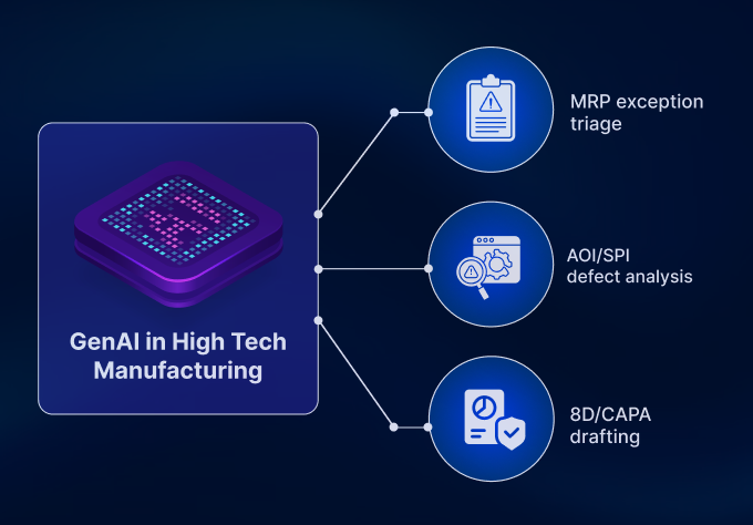
Generative AI in High-Tech Manufacturing: Operating Model, Use Cases, Governance, and Future Trends
In high-tech manufacturing environments, generative and agentic AI can interpret, synthesize, and generate structured outputs from technical and operational information.

Comparison of Large Language Models (LLMs): A detailed analysis
Large Language Models (LLMs) have emerged as a cornerstone in the advancement of artificial intelligence, transforming our interaction with technology and our ability to process and generate human language.

Actionable AI: An evolution from Large Language Models to Large Action Models
Actionable AI not only analyzes data but also uses those insights to drive specific, automated actions.

Federated learning: Unlocking the potential of secure, distributed AI
Federated learning aims to train a unified model using data from multiple sources without the need to exchange the data itself.

Optimize to actualize: The impact of hyperparameter tuning on AI
Hyperparameter tuning is a critical aspect of machine learning, involving configuration variables that significantly influence the training process of a model.

Journey to AGI: Exploring the next frontier in artificial intelligence
Artificial General Intelligence represents a significant leap in the evolution of artificial intelligence, characterized by capabilities that closely mirror the intricacies of human intelligence.

How attention mechanism’s selective focus fuels breakthroughs in AI
The attention mechanism significantly enhances the model’s capability to understand, process, and predict from sequence data, especially when dealing with long, complex sequences.

What is LLMOps? Exploring the fundamentals and significance of large language model operations
LLMOps, or Large Language Model Operations, encompass the practices, techniques, and tools used to deploy, monitor, and maintain LLMs effectively.

Ensuring ML model accuracy and adaptability through model validation techniques
As businesses lean heavily on data-driven decisions, it’s not an exaggeration to say that a company’s success may very well hinge on the strength of its model validation techniques.